DB Scan Clustering Numerical

DBSCAN Clustering Algorithm: A Numerical Solution Explained
DBSCAN clustering (Density-Based Spatial Clustering of Applications with Noise) is a powerful unsupervised machine learning algorithm that groups data points based on density rather than distance to a centroid. Unlike K-Means clustering, DBSCAN clustering can discover clusters of arbitrary shape and naturally handles noise points — outliers that don't belong to any cluster.
In this numerical solution, we'll work through a 12-point dataset step by step, classifying every point as a core point, border point, or noise point using ε = 1.9 and MinPts = 4.
DBSCAN Concepts Recap
Before jumping into the data, here are the three key definitions that drive every classification decision:
ε (epsilon): Radius of the neighborhood around a point
MinPts: Minimum number of points (including the point itself) required within ε to qualify as a core point
Core Point: Has ≥ MinPts neighbors within ε distance — the backbone of any cluster in data clustering
Border Point: Fewer than MinPts neighbors, but lies within ε of a core point
Noise Point: Neither a core point nor reachable from any core point — treated as an outlier
These three categories are what DBSCAN clustering uses to separate meaningful structure from noise in any dataset.
Given Parameters
ε = 1.9
MinPts = 4
Dataset: 12 Points on a 2D Grid
Point | x | y |
|---|---|---|
P1 | 7 | 4 |
P2 | 6 | 4 |
P3 | 5 | 6 |
P4 | 4 | 2 |
P5 | 6 | 3 |
P6 | 5 | 2 |
P7 | 3 | 3 |
P8 | 4 | 5 |
P9 | 6 | 5 |
P10 | 3 | 6 |
P11 | 4 | 4 |
P12 | 8 | 2 |
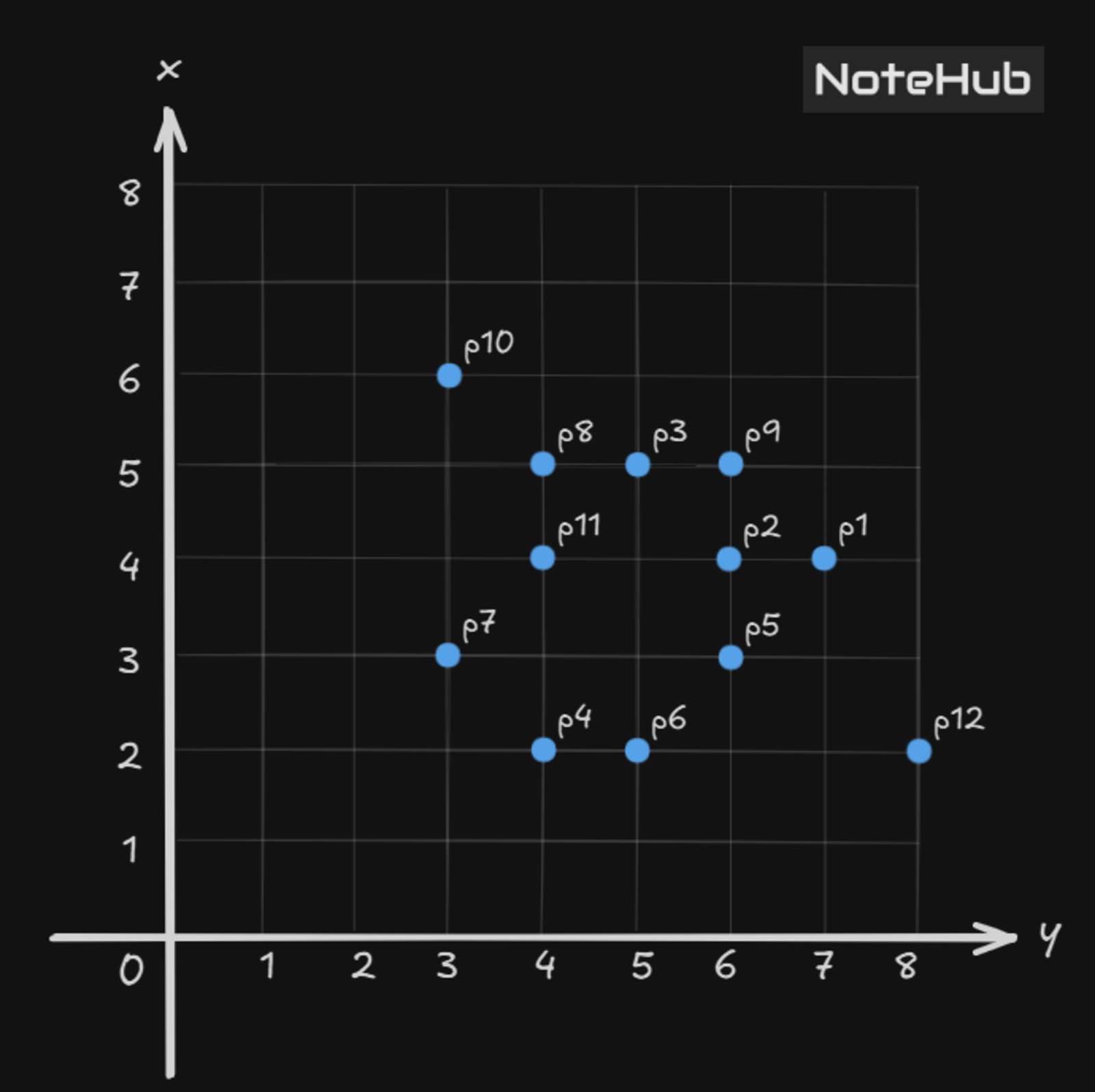
Step 1: Euclidean Distance Matrix
The Euclidean distance between any two points A and B is:
We compute this for all 12×12 pairs to determine which points fall within ε = 1.9 of each other.
12×12 Distance Matrix (rounded to 2 decimals)
P1 | P2 | P3 | P4 | P5 | P6 | P7 | P8 | P9 | P10 | P11 | P12 | |
|---|---|---|---|---|---|---|---|---|---|---|---|---|
P1 | 0.00 | 1.00 | 2.83 | 3.61 | 1.41 | 2.83 | 4.12 | 3.16 | 1.41 | 4.47 | 3.00 | 2.24 |
P2 | 1.00 | 0.00 | 2.24 | 2.83 | 1.00 | 2.24 | 3.16 | 2.24 | 1.00 | 3.61 | 2.00 | 2.83 |
P3 | 2.83 | 2.24 | 0.00 | 4.12 | 3.16 | 4.00 | 3.61 | 1.41 | 1.41 | 2.00 | 2.24 | 5.00 |
P4 | 3.61 | 2.83 | 4.12 | 0.00 | 2.24 | 1.00 | 1.41 | 3.00 | 3.61 | 4.12 | 2.00 | 4.00 |
P5 | 1.41 | 1.00 | 3.16 | 2.24 | 0.00 | 1.41 | 3.00 | 2.83 | 2.00 | 4.24 | 2.24 | 2.24 |
P6 | 2.83 | 2.24 | 4.00 | 1.00 | 1.41 | 0.00 | 2.24 | 3.16 | 3.16 | 4.47 | 2.24 | 3.00 |
P7 | 4.12 | 3.16 | 3.61 | 1.41 | 3.00 | 2.24 | 0.00 | 2.24 | 3.61 | 3.00 | 1.41 | 5.10 |
P8 | 3.16 | 2.24 | 1.41 | 3.00 | 2.83 | 3.16 | 2.24 | 0.00 | 2.00 | 1.41 | 1.00 | 5.00 |
P9 | 1.41 | 1.00 | 1.41 | 3.61 | 2.00 | 3.16 | 3.61 | 2.00 | 0.00 | 3.16 | 2.24 | 3.61 |
P10 | 4.47 | 3.61 | 2.00 | 4.12 | 4.24 | 4.47 | 3.00 | 1.41 | 3.16 | 0.00 | 2.24 | 6.40 |
P11 | 3.00 | 2.00 | 2.24 | 2.00 | 2.24 | 2.24 | 1.41 | 1.00 | 2.24 | 2.24 | 0.00 | 4.47 |
P12 | 2.24 | 2.83 | 5.00 | 4.00 | 2.24 | 3.00 | 5.10 | 5.00 | 3.61 | 6.40 | 4.47 | 0.00 |
Any cell value ≤ 1.9 means those two points are neighbors. Each point also counts itself, so a point needs 3 external neighbors to reach MinPts = 4.
Step 2: Classify Each Point
Core Point Condition
≥ 4 neighbors (including itself) within distance ≤ 1.9
Border Point Condition
Fewer than 4 neighbors, but lies within ε of at least one core point
Noise Point Condition
Neither a core point nor within ε of any core point
P1 (7, 4)
Neighbors within ε = 1.9: P2 (1.00), P5 (1.41), P9 (1.41) → plus itself = 4
✅ 4 ≥ MinPts → Core Point
P2 (6, 4)
Neighbors within ε = 1.9: P1 (1.00), P5 (1.00), P9 (1.00) → plus itself = 4
✅ 4 ≥ MinPts → Core Point
P3 (5, 6)
Neighbors within ε = 1.9: P8 (1.41), P9 (1.41) → plus itself = 3
⚠️ 3 < MinPts → not a core point. But P3 lies within ε of P8 and P9, both core points.
Border Point (of P8, P9)
P4 (4, 2)
Neighbors within ε = 1.9: P6 (1.00), P7 (1.41) → plus itself = 3
❌ 3 < MinPts. P4's neighbors (P6, P7) are not core points, so P4 is unreachable from any core.
❌ Noise Point
P5 (6, 3)
Neighbors within ε = 1.9: P1 (1.41), P2 (1.00), P6 (1.41) → plus itself = 4
✅ 4 ≥ MinPts → Core Point
P6 (5, 2)
Neighbors within ε = 1.9: P4 (1.00), P5 (1.41) → plus itself = 3
⚠️ 3 < MinPts → not a core point. But P6 lies within ε of P5, a core point.
Border Point (of P5)
P7 (3, 3)
Neighbors within ε = 1.9: P4 (1.41), P11 (1.41) → plus itself = 3
❌ 3 < MinPts. Neither P4 nor P11 are core points, so P7 is not reachable from any core.
❌ Noise Point
P8 (4, 5)
Neighbors within ε = 1.9: P3 (1.41), P10 (1.41), P11 (1.00) → plus itself = 4
✅ 4 ≥ MinPts → Core Point
P9 (6, 5)
Neighbors within ε = 1.9: P1 (1.41), P2 (1.00), P3 (1.41) → plus itself = 4
✅ 4 ≥ MinPts → Core Point
P10 (3, 6)
Neighbors within ε = 1.9: P8 (1.41) → plus itself = 2
⚠️ 2 < MinPts → not a core point. But P10 lies within ε of P8, a core point.
Border Point (of P8)
P11 (4, 4)
Neighbors within ε = 1.9: P7 (1.41), P8 (1.00) → plus itself = 3
⚠️ 3 < MinPts → not a core point. But P11 lies within ε of P8, a core point.
Border Point (of P8)
P12 (8, 2)
Neighbors within ε = 1.9: none → plus itself = 1
❌ 1 < MinPts, and no core point is within ε of P12.
❌ Noise Point
Final Classification Summary
Type | Points |
|---|---|
Core | P1, P2, P5, P8, P9 |
Border | P3, P6, P10, P11 |
Noise | P4, P7, P12 |
Full Point-wise Table
Point | Neighbors (within ε=1.9) | Count | Type |
|---|---|---|---|
P1 | P2, P5, P9 | 4 | ✅ Core |
P2 | P1, P5, P9 | 4 | ✅ Core |
P3 | P8, P9 | 3 | ⚠️ Border (P8, P9) |
P4 | P6, P7 | 3 | ❌ Noise |
P5 | P1, P2, P6 | 4 | ✅ Core |
P6 | P4, P5 | 3 | ⚠️ Border (P5) |
P7 | P4, P11 | 3 | ❌ Noise |
P8 | P3, P10, P11 | 4 | ✅ Core |
P9 | P1, P2, P3 | 4 | ✅ Core |
P10 | P8 | 2 | ⚠️ Border (P8) |
P11 | P7, P8 | 3 | ⚠️ Border (P8) |
P12 | None | 1 | ❌ Noise |
Key Takeaway
This numerical solution demonstrates how DBSCAN clustering builds clusters purely from density reachability — no preset number of clusters required. The five core points (P1, P2, P5, P8, P9) anchor two overlapping density regions, the four border points attach to those regions at the edges, and three noise points (P4, P7, P12) remain isolated outliers.
This behavior is what makes DBSCAN clustering especially useful in real-world machine learning tasks where cluster shapes are irregular and outliers are expected. To understand the theory behind this algorithm before working numericals, see the DBSCAN Clustering concept note. For comparison with centroid-based data clustering, refer to K-Means Clustering.
Related Notes:
DBSCAN Clustering (Theory) → · K-Means Clustering → · Dimensionality Reduction