Artificial Neural Network

May 13, 2025

Updated 1 month ago

4 min read

Artificial Neural Network (ANN) — Architecture, Neurons & Activation Functions

Artificial Neural Networks (ANNs) are the backbone of modern machine learning. Before jumping into advanced models like CNN or RNN, it's important to understand how a basic neural network is structured — starting from how biological neurons inspire the design, to how activation functions introduce non-linearity that makes learning possible.

Brain and Perceptrons

Biological learning systems are built from a very complex web of interconnected neurons. The human brain has an immensely connected network of approximately 100 billion $(1 0^{11})$ neurons, each connected on average to 1,000 $(1 0^{3})$ other neurons.

Even though neuron transmission speeds are much slower than computer processing speeds, the brain's massive parallelism makes it extremely powerful for learning and decision-making tasks.

The Perceptron — the simplest form of an artificial neural network — was directly inspired by this biological design.

Artificial Neurons

An artificial neuron is a mathematical function conceived as a model of a biological neuron. Artificial neurons are the elementary units of an artificial neural network (ANN).

This artificial neuron receives one or more inputs and sums them to produce an output. Each input is individually weighted, and the sum is passed through a function known as the activation function or transfer function.

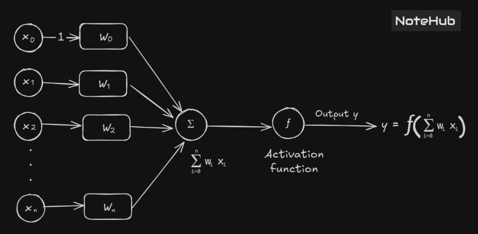
Artificial neural network showing inputs, weights, summation, and activation function producing output.

Terminology

Symbol	Meaning
$x$	Input signal
$w$	Weights associated with inputs
$x_{0}$	Bias input (constant value of 1)
$w_{0}$	Weight associated with $x_{0}$ (bias weight)
$\sum w x$	Weighted sum of input signals
$f (\sum w x)$	Activation function output
$y$	Output signal

The output of a neuron is computed as:

y = i = 0 \sum n w_{i} x_{i}

Activation Functions

In artificial neural networks, the activation function takes the weighted sum as input and decides the output of the neuron. Without activation functions, a neural network — no matter how deep — would behave like a single linear transformation. Activation functions introduce non-linearity, which is what allows networks to learn complex patterns.

For a deeper look at how these functions interact with training, see the Loss Function and Gradient Descent posts.

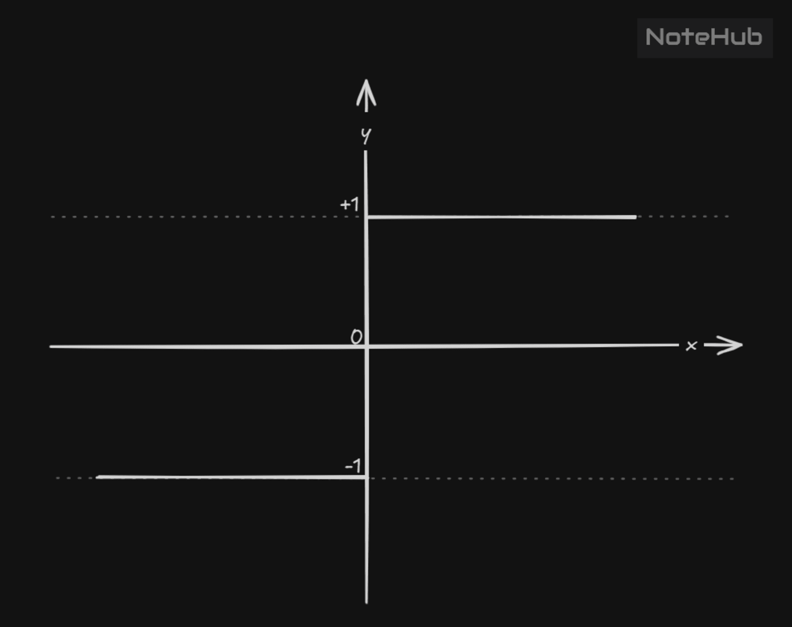
1. Threshold Activation Function

The threshold activation function produces a binary output based on whether the input crosses zero:

f (x) = {1 if x > 0 - 1 if x \leq 0

Threshold activation function graph showing output switching between −1 and +1 based on input.

2. Unit Step Function

Sometimes the threshold activation function is also defined as the unit step function, in which the output range shifts from {-1, 1} to {0, 1}:

f (x) = {1 if x \geq 00 if x < 0

3. Sigmoid Activation Function (Logistic Function)

One of the most commonly used activation functions is the sigmoid (or logistic) function. It maps any input to a smooth output between 0 and 1, making it especially useful for binary classification problems.

It is defined as:

f (z) = \frac{1}{1 + e ^{- z}}

Sigmoid activation function curve mapping input values smoothly between 0 and 1.

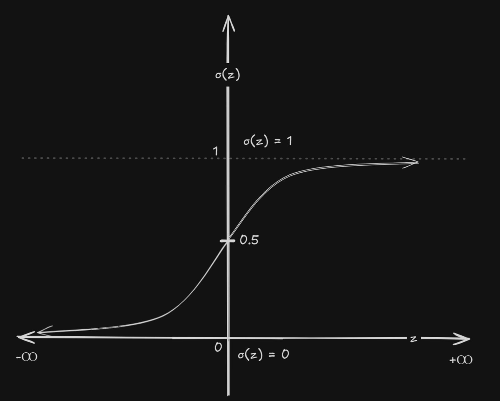
You can see sigmoid used in practice in the Logistic Regression post.

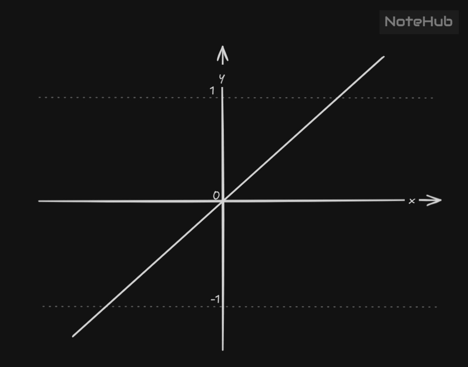
4. Linear Activation Function

The linear activation function outputs a value directly proportional to the input:

f (x) = m x + c

Linear activation function graph showing straight-line relationship between input and output.

5. Piecewise Saturated Linear Activation Function

This function behaves linearly within a defined range and saturates (clips) outside it:

f (x) = {0 if x < x_{min} m x + c if x_{min} \leq x \leq x_{ma x} 0 if x > x_{ma x}

6. Gaussian Activation Function

The Gaussian activation function is defined as:

f (x) = \frac{1}{σ 2 π} e^{- \frac{x ^{2}}{2 σ ^{2}}}

Where:

$σ$ is the standard deviation
$π$ is the mathematical constant Pi
$e^{- \frac{x ^{2}}{2 σ ^{2}}}$ ensures the Gaussian (bell-curve) shape

This function is commonly used in radial basis function (RBF) networks and probabilistic models.

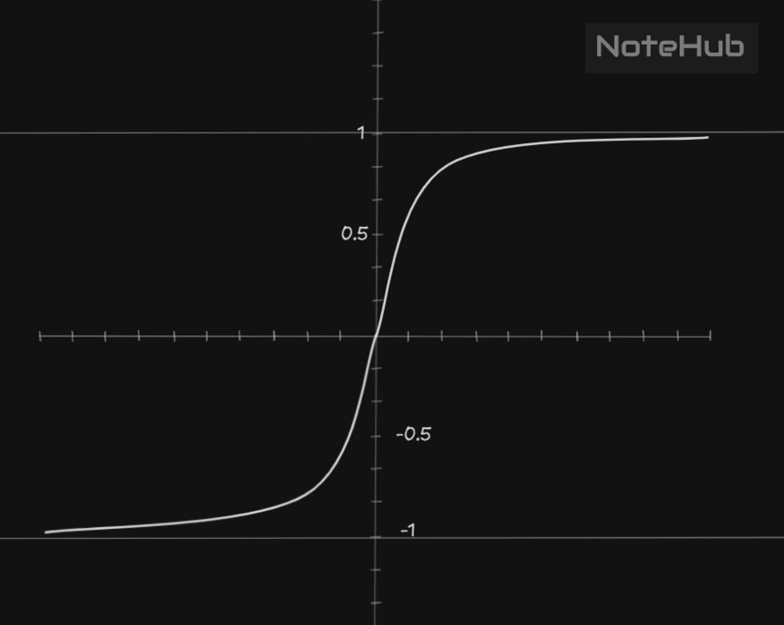
7. Hyperbolic Tangent (tanh) Activation Function

The tanh function is similar to sigmoid but outputs values in the range [-1, 1], making it zero-centered — which often helps with training stability.

It is defined as:

f (x) = \frac{e ^{x} - e ^{- x}}{e ^{x} + e ^{- x}}

Tanh activation function graph showing output range between −1 and +1 with smooth S-shaped curve.

8. ReLU (Rectified Linear Unit)

The Rectified Linear Unit (ReLU) is the most widely used activation function in modern deep learning, especially in Convolutional Neural Networks (CNN).

It is defined as:

f (x) = max (0, x)

Which can also be written as:

f (x) = {x 0 if x > 0 if x \leq 0

Why ReLU? Sigmoid and tanh both suffer from the vanishing gradient problem — during backpropagation, gradients become extremely small, slowing down learning. ReLU avoids this by outputting the input directly for positive values, keeping gradients healthy. See Gradient Descent for more on how this affects training.

Quick Comparison

Activation Function	Output Range	Use Case
Threshold	{-1, 1}	Binary decisions
Unit Step	{0, 1}	Simple binary output
Sigmoid	(0, 1)	Binary classification, output layer
Linear	$(- \infty, + \infty)$	Regression output layer
Piecewise Linear	Clipped linear	Custom saturation range
Gaussian	(0, 1]	RBF networks, probabilistic models
Tanh	(-1, 1)	Hidden layers, zero-centered output
ReLU	$[0, + \infty)$	Hidden layers in deep networks, CNN

What's Next?

Now that you understand how a single neuron works and how activation functions shape its output, the next step is understanding how networks of neurons learn — through loss minimization and backpropagation.

Loss Function — how a network measures its own error
Gradient Descent — how it learns by minimizing that error
Perceptron — the simplest neural network building block
Convolutional Neural Network (CNN) — applying neural networks to image data