Branch and Bound Technique

Branch and Bound: Smarter Exhaustive Search

Backtracking explores. Branch and Bound explores — but with a calculator in hand, ready to stop the moment a path can't possibly win.

Here's the honest version of what most DAA courses teach: backtracking is "smart brute force" because it prunes dead ends. Branch and Bound is presented right after as "even smarter" — and then the explanation gets mathematical fast, and most students nod and move on.

But there's a simpler way to think about it.

Imagine you're looking for the cheapest flight route from Delhi to New York with layovers. You're exploring options one by one. At some point, you're looking at a partial route — Delhi → Dubai → London — and the cost so far is already ₹95,000. You know the cheapest remaining leg (London → New York) costs at least ₹40,000. So your best possible total on this path is ₹1,35,000.

But you already found a complete route that costs ₹1,20,000.

Do you keep exploring this branch? No. You kill it immediately.

That's Branch and Bound. The "bound" is the ₹1,35,000 estimate. The "branch" is the part where you built the partial route. The insight is: you don't need to reach the end of a bad path to know it's bad.

What Is the State-Space Tree?

Branch and Bound operates on a state-space tree — the same implicit graph that backtracking uses.

Each node represents a partial solution (a decision made so far). Each edge represents a choice (include this item / take this path / assign this value). Each leaf represents a complete solution.

The tree is called "implicit" because we never build it fully — it would be exponentially large. Instead, we generate nodes on demand and discard entire subtrees the moment they're provably suboptimal.

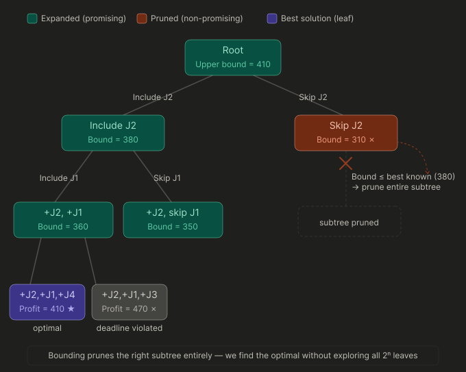
Without pruning, this tree has $2^n$ leaves for $n$ items. With a good bounding function, most branches die early.

The Core Idea: Bounding Function

The bounding function is the heart of Branch and Bound. It answers one question at every node:

"Even in the best possible scenario from here — what's the most (or least) I could achieve?"

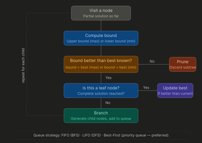
For a maximisation problem (like 0/1 Knapsack): compute an upper bound at each node. If the upper bound is less than or equal to the best complete solution found so far → prune.

For a minimisation problem (like TSP, shortest path): compute a lower bound at each node. If the lower bound is greater than or equal to the best solution found so far → prune.

Promising vs Non-Promising Nodes

This is the exact same vocabulary as backtracking — promising/non-promising — but the reason a node is non-promising is different. In backtracking, a node is dead because it violates a constraint. In Branch and Bound, a node is dead because its ceiling isn't high enough (or its floor isn't low enough).

What Makes a Good Bounding Function?

This is where Branch and Bound becomes an art, not just an algorithm.

The bounding function must be:

1. Accurate — A loose bound prunes nothing. If your upper bound for every node is always "infinity," you'll explore the entire tree. The tighter the bound, the more pruning occurs.

2. Simple — A bound that takes $O(2^n)$ to compute defeats the purpose. The bound computation should be fast (ideally $O(n)$ or $O(n\log n)$), otherwise the overhead kills the speedup.

This tension — accuracy vs. simplicity — is the real design challenge. In the 0/1 Knapsack problem, a common upper bound is the fractional relaxation: assume you can take fractions of items (like Fractional Knapsack). This overestimates the true maximum, but it's computable in $O(n\log n)$ and prunes aggressively.

Branch and Bound vs Backtracking

Both explore a state-space tree. The difference is when and why they prune:

Backtracking says: "This path is illegal — stop." Branch and Bound says: "This path is legal, but it can't possibly beat what I already have — stop."

You can combine both: prune infeasible nodes (backtracking-style) and prune suboptimal nodes (B&B-style). Many real implementations do exactly this.

The Search Strategy: Which Node to Expand Next?

Once you have a tree with multiple promising nodes, you need a strategy for which one to explore first. This is the search strategy, and it matters more than it looks:

FIFO (Queue — BFS order):

• Explores level by level

• Finds short solutions first

• High memory usage (stores entire frontier)

LIFO (Stack — DFS order):

• Dives deep first, like backtracking

• Low memory usage

• May explore bad branches before good ones

Best-First Search (Priority Queue):

• Always expands the node with the best bound

• Most efficient in practice — jumps toward promising regions

• Standard choice for Branch and Bound

Best-First is typically implemented with a max-heap (maximisation) or min-heap (minimisation). The node with the best bound is always at the top.

Complexity

Branch and Bound doesn't have a clean closed-form complexity — it depends entirely on how good your bounding function is.

This is why the bounding function design is non-negotiable. A weak bound gives you exponential runtime with extra overhead. A tight bound can make an intractable problem tractable for realistic input sizes.

Where It's Actually Used

Branch and Bound isn't academic. It's inside:

• Integer Linear Programming solvers (CPLEX, Gurobi) — industrial optimisation

• TSP solvers — route optimisation in logistics

• Chess and game tree search — combined with alpha-beta pruning (which is a form of B&B)

• Job scheduling on multiple machines

• VLSI chip design — placement and routing problems

The 0/1 Knapsack and TSP are the canonical teaching examples, but the pattern scales to real-world NP-hard problems where exact solutions are needed within practical time limits.

Quick Self-Test

• Q1: What's the key difference between how backtracking and Branch and Bound decide to prune a node?

• Q2: For a minimisation problem, when do you prune a node?

• Q3: Why does the bounding function need to be both accurate and simple — why isn't accuracy alone enough?

• Q4: Why is Best-First Search preferred over DFS for Branch and Bound in practice?

(Answers: Backtracking prunes on constraint violation (feasibility); B&B prunes on bound comparison (optimality). Prune when lower_bound ≥ best_complete_solution_so_far. A complex-but-accurate bound can cost more to compute than the savings from pruning — the net result is slower than brute force. Best-First explores the most promising node first, reaching a good solution faster, which tightens the bound used for pruning all subsequent nodes.)

Related Notes

• Traveling Salesman Problem — Exact Solution via Branch and Bound

• Assignment Problem — Branch and Bound with pruning

• Greedy Approach for Algorithm Design — greedy is fast but approximate; B&B is exact but slower. Know when to use which

• Dynamic Programming & 0/1 Knapsack — DP solves 0/1 Knapsack exactly; B&B is the alternative exact approach worth comparing

• Fraction Knapsack — the fractional relaxation used inside the B&B bounding function for Knapsack

• Graph — state-space trees are graphs; understanding graph traversal is prerequisite

• Dijkstra's Algorithm — Best-First Search in B&B is structurally similar to Dijkstra's priority-queue expansion

• All Pairs Shortest Path (Floyd's) — TSP uses B&B; Floyd's is an exact DP alternative for shortest paths

• Full DAA Notes Index

External References

• Branch and Bound — Wikipedia — formal definition, history, and variants

• CP-Algorithms: Branch and Bound — applied B&B patterns with complexity analysis

• CLRS Chapter 35 — NP-completeness context: why B&B exists as an exact solver for hard problems

• Visualgo — graph traversal animations that build the state-space tree intuition

Part of the DAA Design and Analysis series on NoteHub.