BFS/DFS

BFS and DFS — Two Ways to Get Lost in a Graph (and Find Your Way Back)
Everyone teaches BFS and DFS with grids and queues. Most explanations feel like reading a dictionary. This one starts with a question you've actually faced in real life.
Start Here: The Maze Problem
You're standing at the entrance of a maze. You want to find the exit.
You have two strategies:
Strategy 1 — The Cautious Explorer:
You don't go deep into any single path. Instead, you explore everything close to you first — all paths at distance 1, then all paths at distance 2, then distance 3... You're basically expanding outward like a ripple in water.
Strategy 2 — The Reckless Adventurer:
You pick one corridor and go as deep as you can. Hit a dead end? Backtrack. Take the next corridor. Go as deep as you can again. Repeat.
That's it. That's BFS and DFS.
No queues yet. No visited arrays yet. Just two philosophies of exploration.
BFS — Breadth First Search
"Explore all neighbours before going deeper."
BFS is the cautious explorer. It processes nodes level by level.
How It Works
Start at the source node. Mark it visited.
Add it to a queue.
While the queue is not empty:
Dequeue the front node
Visit all its unvisited neighbours
Mark them visited and enqueue them
The queue enforces order — whoever came first gets explored first. FIFO (First In, First Out).
Pseudocode
BFS(Graph G, start node s):
    create queue Q
    mark s as visited
    enqueue s into Q

    while Q is not empty:
        u = dequeue(Q)
        process(u)
        for each neighbour v of u:
            if v is not visited:
                mark v as visited
                enqueue v into Q
Visualizing BFS on a Graph
Graph:
    1 — 2 — 5
    |   |
    3 — 4

BFS from node 1:

Level 0: [1]
Level 1: [2, 3]        ← neighbours of 1
Level 2: [4, 5]        ← neighbours of 2 and 3 (not yet visited)

Order visited: 1 → 2 → 3 → 4 → 5
BFS visits nodes in waves. All nodes at distance d are visited before any node at distance d+1.
Time and Space Complexity
BFS | |
|---|---|
Time | O(V + E) |
Space | O(V) — for the visited array and queue |
Where V = vertices, E = edges.
DFS — Depth First Search
"Go as deep as possible. Backtrack only when stuck."
DFS is the reckless adventurer. It dives into one path completely before trying another.
How It Works
Recursive version (the cleaner one to understand):
Visit the current node. Mark it visited.
For each unvisited neighbour, recursively call DFS on it.
The call stack does the backtracking for you automatically — when a recursive call returns, you're back at the previous node.
Iterative version uses an explicit stack instead of recursion.
Pseudocode (Recursive)
DFS(Graph G, node u):
    mark u as visited
    process(u)
    for each neighbour v of u:
        if v is not visited:
            DFS(G, v)
Pseudocode (Iterative)
DFS_Iterative(Graph G, start node s):
    create stack S
    push s into S

    while S is not empty:
        u = pop(S)
        if u is not visited:
            mark u as visited
            process(u)
            for each neighbour v of u:
                if v is not visited:
                    push v into S
Visualizing DFS on a Graph
Same graph:
    1 — 2 — 5
    |   |
    3 — 4

DFS from node 1 (assuming neighbours visited left-to-right):

1 → go to 2
    2 → go to 5
        5 → dead end, backtrack
    2 → backtrack (4 is next)
        4 → go to 3
            3 → already explored (1 is visited, backtrack)
        4 → backtrack
    2 → backtrack
1 → done

Order visited: 1 → 2 → 5 → 4 → 3
DFS goes deep first, backtracks, then explores the next branch.
Time and Space Complexity
DFS | |
|---|---|
Time | O(V + E) |
Space | O(V) — recursion stack depth in worst case |
BFS vs DFS — Side by Side
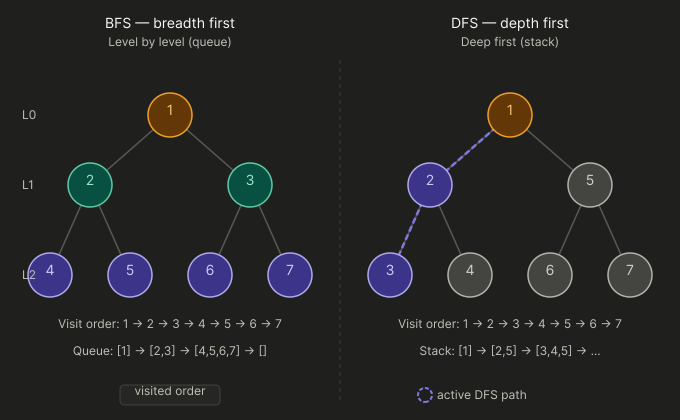
Feature | BFS | DFS |
|---|---|---|
Data Structure | Queue (FIFO) | Stack (LIFO) / Recursion |
Traversal style | Level by level | Branch by branch |
Finds shortest path? | ✅ Yes (unweighted graphs) | ❌ No |
Memory usage | Higher (stores entire frontier) | Lower (stores one path) |
Completeness | Complete (always finds solution if exists) | Complete for finite graphs |
Best for | Shortest path, nearest node | Cycle detection, topological sort, maze solving |
One thing that trips people up: both have O(V + E) time complexity. The difference is in which path they find and how much memory they use, not how fast they are.
When to Use Which — The Real Answer
This is the question most textbooks dodge.
Use BFS when:
You need the shortest path in an unweighted graph ("minimum number of hops")
You're doing level-order traversal of a tree
You need to find all nodes within a certain distance
Example problems: social network degrees of separation, word ladder, minimum moves in a puzzle
Use DFS when:
You need to detect cycles in a graph
You're doing topological sorting (prerequisite ordering)
You're solving maze/backtracking problems
You need to find connected components
You're checking if a graph is bipartite
Example problems: Sudoku solver, N-Queens, detecting deadlocks
A good rule of thumb: if the problem says "minimum steps" or "minimum distance" — think BFS. If it says "all possible paths" or "check if exists" — think DFS.
Applications in DAA — What Actually Shows Up
1. Cycle Detection
Undirected graph — DFS: If you visit a neighbour that's already visited and it's not your parent in the DFS tree, there's a cycle.
Directed graph — DFS with three colors:
White: not yet visited
Gray: currently being processed (in the recursion stack)
Black: completely processed
If you hit a gray node during DFS, there's a back edge → cycle exists.
2. Topological Sort (DFS-based)
For a Directed Acyclic Graph (DAG), topological order is a linear ordering of vertices such that for every edge u → v, u appears before v.
DFS approach: Run DFS. When a node is fully processed (all its neighbours explored), push it to a stack. The stack gives reverse topological order.
DFS_Topo(node u):
    mark u as visited
    for each neighbour v of u:
        if v is not visited:
            DFS_Topo(v)
    push u to result stack
3. Connected Components
Run DFS/BFS from every unvisited node. Each new "start" is a new connected component. Count the number of times you start a fresh traversal — that's your answer.
4. Shortest Path in Unweighted Graphs
BFS naturally gives shortest paths. During BFS, maintain a distance[] array:
distance[source] = 0
when you enqueue a node v from node u:
    distance[v] = distance[u] + 1
At the end, distance[v] is the minimum number of edges from source to v.
The Visited Array — Why It Matters
New learners sometimes forget to mark nodes as visited. Here's what happens:
Graph: 1 — 2 — 1 (cycle)

Without visited tracking:
1 → 2 → 1 → 2 → 1 → 2 → ... infinite loop
Always mark a node as visited before (or as soon as) you add it to the queue or start its DFS. In BFS especially, mark it when enqueuing — not when dequeuing — or you'll add the same node multiple times.
DFS Tree Terminology (Comes Up in Exams)
When DFS runs on a graph, it produces a DFS tree. The edges are classified:
Edge Type | Description |
|---|---|
Tree edge | Edge used to discover a new node |
Back edge | Edge to an ancestor in DFS tree (indicates cycle in directed graph) |
Forward edge | Edge to a descendant that's already visited (directed graphs only) |
Cross edge | Edge to a node in a different DFS subtree (directed graphs only) |
In an undirected graph, only tree edges and back edges exist.
Common Mistakes in Exams
1. Using DFS for shortest path
DFS does not guarantee shortest path. It finds a path, not the shortest path. Use BFS for unweighted, Dijkstra for weighted.
2. Confusing iterative DFS with BFS
Both look similar in code — one uses a stack, one uses a queue. Swap them and you've accidentally written BFS when you meant DFS.
3. Forgetting to mark visited before enqueuing in BFS
Classic bug that causes nodes to be processed multiple times. Mark when you push, not when you pop.
4. DFS on disconnected graphs
A single DFS call from one node won't cover all nodes if the graph is disconnected. You need to call DFS from every unvisited node.
Quick Revision Cheatsheet
BFS:
├── Data structure: Queue
├── Order: Level by level (nearest first)
├── Shortest path: YES (unweighted)
├── Use for: Shortest path, level-order, nearest node
└── Time: O(V + E), Space: O(V)

DFS:
├── Data structure: Stack / Recursion
├── Order: Deep first, then backtrack
├── Shortest path: NO
├── Use for: Cycle detection, topo sort, connected components
└── Time: O(V + E), Space: O(V)

Both:
└── Require a visited[] array to avoid infinite loops
Related Notes
Graph Theory — Foundation — understand graph representations before diving into traversals
Dijkstra's Algorithm — BFS extended to weighted graphs
MST — Kruskal's & Prim's — graph algorithms that use greedy + traversal logic
All Pairs Shortest Path — Floyd-Warshall — when you need shortest paths between all node pairs
Greedy Approach for Algorithm Design — the philosophy behind Prim's and Dijkstra
Binary Search Tree — tree traversals are a special case of DFS
Dynamic Programming – 0/1 Knapsack — another fundamental DAA technique
DAA PYQ — Previous Year Questions — practice BFS/DFS questions that actually showed up in exams
Asymptotic Notation — understand what O(V+E) really means
External References
Part of the DAA (Design and Analysis of Algorithms) series.