Polynomial Regression

Mar 3, 2025

Updated 1 day ago

3 min read

Polynomial Regression Explained Simply

What is Polynomial Regression?

Not every relationship in data follows a straight line. In many real-world situations, data bends, curves, or changes direction. A simple linear regression model cannot accurately capture these patterns.

This is where Polynomial Regression becomes useful.

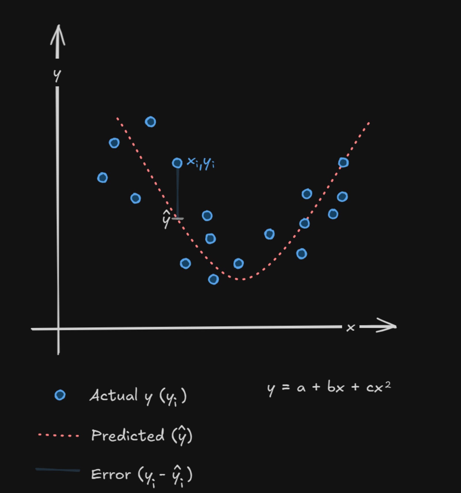
Polynomial regression is a supervised machine learning algorithm used to model non-linear relationships between variables by fitting a curved line instead of a straight one.

For example:

Population growth
Temperature changes
Stock market trends
Sales growth over time

These patterns often form curves rather than straight lines.

Polynomial regression graph showing curved best fit line with actual data points, predicted values, and quadratic equation

Polynomial Equation

A polynomial equation looks like this:

y = f (x) = a_{0} + a_{1} x + a_{2} x^{2} + \dots + a_{n} x^{n}

Where:

$a_{0}, a_{1}, a_{2}, ..., a_{n}$ are constants
$n$ is the degree of the polynomial
$x$ is the input feature
$y$ is the predicted output

If the highest power of $x$ is:

$1$ → Linear Regression
$2$ → Quadratic Polynomial
$3$ → Cubic Polynomial

Example of a second-degree polynomial:

f (x) = a + b x + c x^{2}

img

If $c \neq = 0$ , then the equation represents a curved relationship.

Why Do We Need Polynomial Regression?

Sometimes data points are distributed in a curved pattern, making it impossible for a straight line to fit properly.

Linear regression may produce large prediction errors in such cases.

Polynomial regression solves this problem by fitting a smooth curve that follows the data more accurately.

Example

Suppose we are predicting:

House prices
Company profit
Student performance
Growth rate

The relationship between variables may increase rapidly at first and then slow down later. This creates a curve instead of a straight line.

Training Data

Assume we have $n$ data points:

(x_{1}, y_{1}), (x_{2}, y_{2}), (x_{3}, y_{3}), \dots, (x_{n}, y_{n})

The polynomial regression model predicts:

$\overset{y_{i}}{^} = a + b x_{i} + c x_{i}^{2}$

Where:

$\overset{y}{^}_{i}$ = predicted value
$y_{i}$ = actual value
$(y_{i} - \overset{y_{i}}{^})$ = error

Error Calculation in Polynomial Regression

The model tries to minimize prediction errors.

Square of Error

$e_{i}^{2} = (y_{i} - \overset{y_{i}}{^})^{2}$

Sum of Squared Errors (SSE)

$E = \sum_{i = 1}^{n} (y_{i} - \overset{y_{i}}{^})^{2}$

Substituting $\overset{y_{i}}{^}$ :

$E = \sum_{i = 1}^{n} (y_{i} - a - b x_{i} - c x_{i}^{2})^{2}$

The main goal is:

Find values of $a$ , $b$ , and $c$
Such that total error $E$ becomes minimum

This method is called the Least Squares Method.

Finding Optimal Values of a, b, and c

To minimize the error, we take partial derivatives of $E$ with respect to:

and equate them to zero.

Partial Derivative with Respect to a

We start with:

$E = \sum_{i = 1}^{n} (y_{i} - a - b x_{i} - c x_{i}^{2})^{2}$

Differentiate partially with respect to $a$ :

$\frac{\partial E}{\partial a} = - 2 \sum_{i = 1}^{n} (y_{i} - a - b x_{i} - c x_{i}^{2})$

Set derivative equal to zero:

$\sum_{i = 1}^{n} (y_{i} - a - b x_{i} - c x_{i}^{2}) = 0$

After simplification:

$\overline{y} - a - b \overline{x} - c \overline{x^{2}} = 0$

Partial Derivative with Respect to b

Differentiate partially with respect to $b$ :

$\frac{\partial E}{\partial b} = - 2 \sum_{i = 1}^{n} x_{i} (y_{i} - a - b x_{i} - c x_{i}^{2})$

Equating to zero:

$\sum_{i = 1}^{n} x_{i} (y_{i} - a - b x_{i} - c x_{i}^{2}) = 0$

After simplification:

$\overline{x y} - a \overline{x} - b \overline{x^{2}} - c \overline{x^{3}} = 0$

Partial Derivative with Respect to c

Differentiate partially with respect to $c$ :

$\frac{\partial E}{\partial c} = - 2 \sum_{i = 1}^{n} x_{i}^{2} (y_{i} - a - b x_{i} - c x_{i}^{2})$

Equating to zero:

$\sum_{i = 1}^{n} x_{i}^{2} (y_{i} - a - b x_{i} - c x_{i}^{2}) = 0$

After simplification:

$\overline{x^{2} y} - a \overline{x^{2}} - b \overline{x^{3}} - c \overline{x^{4}} = 0$

Final Normal Equations

After solving all derivatives, we get three equations:

$\overline{y} - a - b \overline{x} - c \overline{x^{2}} = 0$

$\overline{x y} - a \overline{x} - b \overline{x^{2}} - c \overline{x^{3}} = 0$

$\overline{x^{2} y} - a \overline{x^{2}} - b \overline{x^{3}} - c \overline{x^{4}} = 0$

These equations are solved to find the best values of:

which produce the best fitting polynomial curve.

Advantages of Polynomial Regression

Captures curved relationships in data
More flexible than linear regression
Provides better accuracy for non-linear patterns
Useful in trend analysis and forecasting

Disadvantages of Polynomial Regression

Can overfit if degree becomes very large
Sensitive to outliers
Higher computation cost
Harder to interpret compared to linear regression

Applications of Polynomial Regression

Polynomial regression is widely used in:

Stock market prediction
Weather forecasting
Growth analysis
Medical research
Sales forecasting
Population analysis
Engineering simulations

Conclusion

Polynomial regression is an extension of linear regression that helps model curved and complex relationships between variables.

Instead of fitting a straight line, it fits a polynomial curve that better represents real-world data patterns.

By minimizing the sum of squared errors using the least squares method, polynomial regression finds the optimal curve for prediction and analysis.